机器学习第一周
文章目录
【注意】最后更新于 October 5, 2023,文中内容可能已过时,请谨慎使用。
前言
- 近几年机器学习很火,但是我对机器学习的了解仅仅在能做可学习的一种程序,通过大量的数据集训练到达目标,但是内部到达是怎么做的完全不知道。
- 这里决通过
斯坦福大学(coursera)的 machine-learning 免费公开课进行学习,并且把学到的知识整理为一篇一篇博文。 - 第一篇的篇幅主要讲
机器学习的定义,监督学习,无监督学习,线性回归,梯度下降。 - 顺便整理一个专有词对应表。
一、机器学习的定义
Arthur Samuel 的定义
第一个机器学习的定义来自于 Arthur Samuel。他定义机器学习为,在进行特定编程的情况下,给予计算机学习能力的领域。Samuel 的定义可以回溯到 50 年代,他编写了一个西洋棋程序。这程序神奇之处在于,编程者自己并不是个下棋高手。但因为他太菜了,于是就通过编程,让西洋棋程序自己跟自己下了上万盘棋。通过观察哪种布局(棋盘位置)会赢,哪种布局会输,久而久之,这西洋棋程序明白了什么是好的布局,什么样是坏的布局。然后就牛逼大发了,程序通过学习后,玩西洋棋的水平超过了 Samuel。这绝对是令人注目的成果。尽管编写者自己是个菜鸟,但因为计算机有着足够的耐心,去下上万盘的棋,没有人有这耐心去下这么多盘棋。通过这些练习,计算机获得无比丰富的经验,于是渐渐成为了比 Samuel 更厉害的西洋棋手。上述是个有点不正式的定义,也比较古老。
Tom Mitchell 的定义
另一个年代近一点的定义,由 Tom Mitchell 提出,来自卡内基梅隆大学,Tom 定义的机器学习是这么啰嗦的,一个好的学习问题定义如下,他说,一个程序被认为能从经验 E 中学习,解决任务 T,达到性能度量值 P,当且仅当,有了经验 E 后,经过 P 评判,程序在处理 T 时的性能有所提升。我认为他提出的这个定义就是为了压韵在西洋棋那例子中,经验 E 就是程序上万次的自我练习的经验而任务 T 就是下棋。性能度量值 P 呢,就是它在与一些新的对手比赛时,赢得比赛的概率。
阅读资料: What is Machine Learning?
原文
Two definitions of Machine Learning are offered. Arthur Samuel described it as: "the field of study that gives computers the ability to learn without being explicitly programmed." This is an older, informal definition.Tom Mitchell provides a more modern definition: “A computer program is said to learn from experience E with respect to some class of tasks T and performance measure P, if its performance at tasks in T, as measured by P, improves with experience E.”
Example: playing checkers.
E = the experience of playing many games of checkers
T = the task of playing checkers.
P = the probability that the program will win the next game.
In general, any machine learning problem can be assigned to one of two broad classifications:
Supervised learning and Unsupervised learning.
机器学习的两个定义。 Arthur Samuel 将其描述为:“研究领域使计算机无需明确编程即可学习。” 这是一个较旧的非正式定义。
Tom Mitchell 提供了一个更现代的定义:“据说计算机程序从经验 E 中学习某些任务 T 和绩效测量 P,如果它在 T 中的任务中的表现,由 P 测量,随经验 E 而改善。“
示例:玩跳棋。
E = 玩许多跳棋游戏的经验
T = 玩跳棋的任务。
P = 程序赢得下一场比赛的概率。
通常,任何机器学习问题都可以分配到两个广泛的分类之一:
监督学习: 可以被预测的结果无监督学习: 无法预测的结果
二、监督学习
原文
In supervised learning, we are given a data set and already know what our correct output should look like, having the idea that there is a relationship between the input and the output.Supervised learning problems are categorized into “regression” and “classification” problems. In a regression problem, we are trying to predict results within a continuous output, meaning that we are trying to map input variables to some continuous function. In a classification problem, we are instead trying to predict results in a discrete output. In other words, we are trying to map input variables into discrete categories.
Example 1:
Given data about the size of houses on the real estate market, try to predict their price. Price as a function of size is a continuous output, so this is a regression problem.
We could turn this example into a classification problem by instead making our output about whether the house “sells for more or less than the asking price.” Here we are classifying the houses based on price into two discrete categories.
Example 2:
(a) Regression - Given a picture of a person, we have to predict their age on the basis of the given picture
(b) Classification - Given a patient with a tumor, we have to predict whether the tumor is malignant or benign.
在有监督的学习中,我们得到一个数据集,并且已经知道我们的正确输出应该是什么样的,并且认为输入和输出之间存在关系。
监督学习问题分为“回归”和“分类”问题。在回归问题中,我们试图在连续输出中预测结果,这意味着我们正在尝试将输入变量映射到某个连续函数。在分类问题中,我们试图在离散输出中预测结果。换句话说,我们正在尝试将输入变量映射到离散类别。
例 1: 鉴于有关房地产市场房屋面积的数据,请尝试预测房价。作为大小函数的价格是连续输出,因此这是一个回归问题。
我们可以将这个例子变成一个分类问题,而不是让我们的输出关于房子“卖得多于还是低于要价”。在这里,我们将基于价格的房屋分为两个不同的类别。
例 2: (a)回归 - 鉴于一个人的照片,我们必须根据给定的图片预测他们的年龄
(b)分类 - 鉴于患有肿瘤的患者,我们必须预测肿瘤是恶性的还是良性的。
三、无监督学习
原文
Unsupervised learning allows us to approach problems with little or no idea what our results should look like. We can derive structure from data where we don't necessarily know the effect of the variables.We can derive this structure by clustering the data based on relationships among the variables in the data.
With unsupervised learning there is no feedback based on the prediction results.
Example:
Clustering: Take a collection of 1,000,000 different genes, and find a way to automatically group these genes into groups that are somehow similar or related by different variables, such as lifespan, location, roles, and so on.
Non-clustering: The “Cocktail Party Algorithm”, allows you to find structure in a chaotic environment. (i.e. identifying individual voices and music from a mesh of sounds at a cocktail party).
我们可以通过基于数据中变量之间的关系对数据进行聚类来推导出这种结构。
在无监督学习的情况下,没有基于预测结果的反馈。
例: 聚类:收集 1,000,000 个不同基因的集合,并找到一种方法将这些基因自动分组成不同的相似或相关的不同变量组,如寿命,位置,角色等。
非聚类:“鸡尾酒会算法”允许您在混乱的环境中查找结构。 (即在鸡尾酒会上从声音网格中识别个别声音和音乐)。
四、练习 1
原文
- A computer program is said to learn from experience E with respect to some task T and some performance measure P if its performance on T, as measured by P, improves with experience E.Suppose we feed a learning algorithm a lot of historical weather data, and have it learn to predict weather. In this setting, what is T?
- a. The process of the algorithm examining a large amount of historical weather data.
- b. The probability of it correctly predicting a future date’s weather.
- c. The weather prediction task.
- d. None of these.
- The amount of rain that falls in a day is usually measured in either millimeters (mm) or inches. Suppose you use a learning algorithm to predict how much rain will fall tomorrow. Would you treat this as a classification or a regression problem?
- a. Regression
- b. Classification
- Suppose you are working on stock market prediction. You would like to predict whether or not a certain company will win a patent infringement lawsuit (by training on data of companies that had to defend against similar lawsuits). Would you treat this as a classification or a regression problem?
- a. Classification
- b. Regression
- Some of the problems below are best addressed using a supervised learning algorithm, and the others with an unsupervised learning algorithm. Which of the following would you apply supervised learning to? (Select all that apply.) In each case, assume some appropriate dataset is available for your algorithm to learn from.
- a. Given data on how 1000 medical patients respond to an experimental drug (such as effectiveness of the treatment, side effects, etc.), discover whether there are different categories or “types” of patients in terms of how they respond to the drug, and if so what these categories are.
- b. Given genetic (DNA) data from a person, predict the odds of him/her developing diabetes over the next 10 years.
- c. Given a large dataset of medical records from patients suffering from heart disease, try to learn whether there might be different clusters of such patients for which we might tailor separate treatments.
- d. Have a computer examine an audio clip of a piece of music, and classify whether or not there are vocals (i.e., a human voice singing) in that audio clip, or if it is a clip of only musical instruments (and no vocals).
- Which of these is a reasonable definition of machine learning?
- a. Machine learning is the field of allowing robots to act intelligently.
- b. Machine learning is the science of programming computers.
- c. Machine learning is the field of study that gives computers the ability to learn without being explicitly programmed.
- d. Machine learning learns from labeled data.
- 一个计算机程序据说可以从经验
E中学习一些任务T和一些绩效测量P,如果它在T上的表现,用P来衡量,随着经验的提高而提高E。假设我们为学习算法提供了大量的历史天气数据,让它学会预测天气。在这种情况下,什么是T?
- a. 该算法检查大量历史天气数据的过程。
- b. 正确预测未来日期天气的概率。
- c. 天气预报任务。
- d. 都不是。
- 一天中下降的雨量通常以毫米(mm)或英寸为单位。假设您使用学习算法来预测明天将下降多少雨。您会将此视为分类还是回归问题?
- a. 回归
- b. 分类
- 假设您正在进行股市预测。您想预测某家公司是否会赢得专利侵权诉讼(通过培训必须为类似诉讼辩护的公司的数据)。您会将此视为分类还是回归问题?
- a. 分类
- b. 回归
- (hasMany)下面的一些问题最好使用监督学习算法解决,其他问题使用无监督学习算法。您将以下哪项应用监督学习? (选择所有适用的选项。)在每种情况下,假设您的算法可以使用一些适当的数据集来学习。
- a. 根据 1000 名医疗患者对实验药物的反应(如治疗效果,副作用等)的数据,发现患者对药物的反应方式是否存在不同的类别或“类型”,以及如果是这样,这些类别是什么。
- b. 根据一个人的遗传(DNA)数据,预测他/她在未来 10 年内患糖尿病的几率。
- c. 根据患有心脏病的患者的医疗记录的大量数据集,尝试了解是否可能存在不同的这类患者群体,我们可以针对这些患者量身定制单独的治疗方案。
- d. 让计算机检查一段音乐的音频片段,并分类该音频片段中是否存在人声(即,人声唱歌),或者它是否仅是乐器(并且没有人声)的片段。
- 这些是机器学习的合理定义?
- a. 机器学习是允许机器人智能行动的领域。
- b. 机器学习是计算机编程的科学。
- c. 机器学习是一个研究领域,它使计算机无需明确编程即可学习。
- d. 机器学习从标记数据中学习。
答案
c根据机器学习定义中的得等T是目标的任务。a根据以往的数据制作为曲线函数或者直线函数来预测一个值,所以是回归算法。a目标要求明确为是否赢得专利侵权诉讼,所以是分类算法。b, c主要问题是c选项中语言陷阱明明是一个是否有其它分类的说法,如果不注意会以为应该用无监督算法。c这个没啥好说的,自己去翻定义。
五、线性回归算法
原文
To establish notation for future use, we’ll use x(i) to denote the input variables (living area in this example), also called input features, and y(i) to denote the output or target variable that we are trying to predict (price). A pair (x(i),y(i)) is called a training example, and the dataset that we’ll be using to learn—a list of m training examples (x(i),y(i)); i=1,... , m is called a training set. Note that the superscript (i) in the notation is simply an index into the training set, and has nothing to do with exponentiation. We will also use X to denote the space of input values, and Y to denote the space of output values. In this example, X = Y = ℝ.
To describe the supervised learning problem slightly more formally, our goal is, given a training set, to learn a function h : X → Y so that h(x) is a good predictor for the corresponding value of y. For historical reasons, this function h is called a hypothesis. Seen pictorially, the process is therefore like this:
When the target variable that we’re trying to predict is continuous, such as in our housing example, we call the learning problem a regression problem. When y can take on only a small number of discrete values (such as if, given the living area, we wanted to predict if a dwelling is a house or an apartment, say), we call it a classification problem.
为了建立未来使用的符号,我们将使用 x(i) 来表示 输入 变量(在此示例中为生活区域),也称为输入要素,并使用 y(i) 来表示我们试图预测的 输出 或目标变量(价格)。一对 (x(i),y(i)) 被称为训练示例,我们将使用的数据集学习 m 个训练样例列表 (x(i),y(i)); i=1,... ,m 称为训练集数量。请注意,符号中的上标 (i) 只是训练集的索引,与取幂无关。我们还将使用 X 来表示输入值的空间,并使用 Y 来表示输出值的空间。在这个例子中,X = Y = ℝ。
为了更加正式地描述监督学习问题,我们的目标是,在给定训练集的情况下,学习函数 h : X → Y,使得 h(x) 是 y 的对应值的 good 预测器。由于历史原因,该函数 h 被称为假设。从图中可以看出,这个过程是这样的:

当我们试图预测的目标变量是连续的时,例如在我们的住房示例中,我们将学习问题称为回归问题。当 y 只能承受少量离散值时(例如,如果给定生活区域,比如说我们想要预测住宅是房屋还是公寓),我们将其称为分类问题。
六、代价函数定义
原文
We can measure the accuracy of our hypothesis function by using a cost function. This takes an average difference (actually a fancier version of an average) of all the results of the hypothesis with inputs from x’s and the actual output y’s.
To break it apart, it is \frac{1}{2}\bar{x} where \bar{x} is the mean of the squares of h_\theta (x_{i}) - y_{i}, or the difference between the predicted value and the actual value.
This function is otherwise called the Squared error function, or Mean squared error. The mean is halved (\frac{1}{2}) as a convenience for the computation of the gradient descent, as the derivative term of the square function will cancel out the \frac{1}{2} term. The following image summarizes what the cost function does:
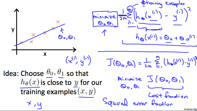
我们可以使用 代价函数 来衡量我们的假设函数的准确性。 这需要假设的所有结果与来自 x's 和实际输出 y's 的输入的平均差异(实际上是平均值的更高版本)。
为了打破它,它是 \frac{1}{2}\bar{x} 其中 \bar{x} 是 h_\theta (x_{i}) - y_{i} 的平方的平均值,或者是预测值之间的差值 和实际价值。
此函数另外称为 平方误差函数 或 均方误差。 平均值减半 (\frac{1}{2}) 为了便于计算梯度下降,因为平方函数的导数项将抵消 \frac{1}{2} 该项。 下图总结了成本函数的作用:
七、代价函数 - 说明 1
原文
If we try to think of it in visual terms, our training data set is scattered on the x-y plane. We are trying to make a straight line (defined by h_θ(x)) which passes through these scattered data points.
Our objective is to get the best possible line. The best possible line will be such so that the average squared vertical distances of the scattered points from the line will be the least. Ideally, the line should pass through all the points of our training data set. In such a case, the value of J(θ_0,θ_1) will be 0. The following example shows the ideal situation where we have a cost function of 0.
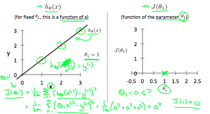
When θ_1=1, we get a slope of 1 which goes through every single data point in our model. Conversely, when θ_1=0.5, we see the vertical distance from our fit to the data points increase.
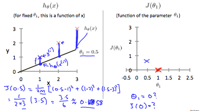
This increases our cost function to 0.58. Plotting several other points yields to the following graph:
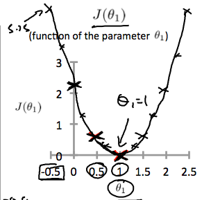
Thus as a goal, we should try to minimize the cost function. In this case, θ_1=1 is our global minimum.
如果我们试图用视觉术语来思考它,我们的训练数据集就会分散在 x-y 平面上。我们试图通过这些分散的数据点建立一条直线(由 h_θ(x) 定义)。
我们的目标是获得最佳线路。最好的线将是这样的,使得来自线的散射点的平均垂直距离将是最小的。理想情况下,该线应该通过我们的训练数据集的所有点。在这种情况下,J(θ_0,θ_1) 的值将为0. 以下示例显示了我们的成本函数为 0 的理想情况。
当θ_1 =1 时,我们得到的斜率为 1,它遍历模型中的每个数据点。相反,当 θ_1=0.5 时,我们看到从拟合到数据点的垂直距离增加。
这使我们的成本函数增加到 0.58。绘制其他几个点会产生如下图:
因此,作为目标,我们应该尽量减少成本函数。在这种情况下,θ_1=1 是我们的全球最低要求。
例子: 训练集数据为:
| |
设定 θ_0 = 0,θ_1 = 1, 函数 h 为 h_θ(x) = 0 + x 所以代价函数的公式会简化为:
用代码表述为:
| |
八、代价函数 - 说明 2
原文
A contour plot is a graph that contains many contour lines. A contour line of a two variable function has a constant value at all points of the same line. An example of such a graph is the one to the right below.

Taking any color and going along the circle, one would expect to get the same value of the cost function. For example, the three green points found on the green line above have the same value for J(θ_0, θ_1) and as a result, they are found along the same line. The circled x displays the value of the cost function for the graph on the left when θ_0 = 800 and θ_1 = -0.15. Taking another h(x) and plotting its contour plot, one gets the following graphs:
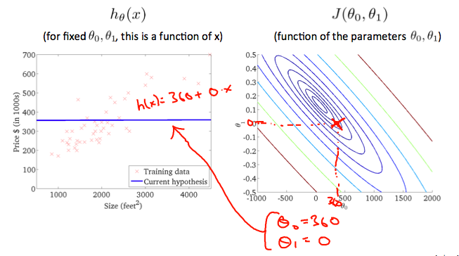
When θ_0 = 360 and θ_1 = 0, the value of J(θ_0, θ_1) in the contour plot gets closer to the center thus reducing the cost function error. Now giving our hypothesis function a slightly positive slope results in a better fit of the data.
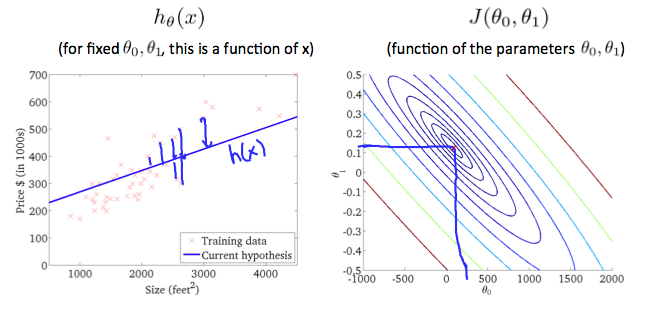
The graph above minimizes the cost function as much as possible and consequently, the result of θ_1 and θ_0 tend to be around 0.12 and 250 respectively. Plotting those values on our graph to the right seems to put our point in the center of the inner most circle.
等高线图是包含许多等高线的图形。双变量函数的等高线在同一行的所有点处具有恒定值。这种图表的一个例子是下面的图表。
采用任何颜色并沿着 circle,人们可以期望得到相同的成本函数值。例如,上面绿线上的三个绿点对于 J(θ_0, θ_1) 具有相同的值,因此,它们沿着同一条线找到。当 θ_0 = 800 和 θ_1 = -0.15 时,带圆圈的 x 显示左侧图形的成本函数的值。取另一个 h(x) 并绘制其等高线图,可以得到以下图表:
当 θ_0 = 360 和 θ_1 = 0 时,等高线图中 J(θ_0, θ_1) 的值越接近中心,从而降低了成本函数误差。现在给出我们的假设函数略微正斜率可以更好地拟合数据。
上图最大限度地降低了成本函数,因此,θ_1 和 θ_0 的结果分别约为 0.12 和 250。在我们的图表右侧绘制这些值似乎将我们的观点置于最内部 圆 的中心。
八、梯度下降
原文
So we have our hypothesis function and we have a way of measuring how well it fits into the data. Now we need to estimate the parameters in the hypothesis function. That's where gradient descent comes in.Imagine that we graph our hypothesis function based on its fields θ_0 and θ_1 (actually we are graphing the cost function as a function of the parameter estimates). We are not graphing x and y itself, but the parameter range of our hypothesis function and the cost resulting from selecting a particular set of parameters.
We put θ_0 on the x axis and θ_1 on the y axis, with the cost function on the vertical z axis. The points on our graph will be the result of the cost function using our hypothesis with those specific theta parameters. The graph below depicts such a setup.
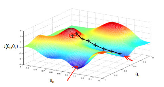
We will know that we have succeeded when our cost function is at the very bottom of the pits in our graph, i.e. when its value is the minimum. The red arrows show the minimum points in the graph.
The way we do this is by taking the derivative (the tangential line to a function) of our cost function. The slope of the tangent is the derivative at that point and it will give us a direction to move towards. We make steps down the cost function in the direction with the steepest descent. The size of each step is determined by the parameter \alpha, which is called the learning rate.
For example, the distance between each star in the graph above represents a step determined by our parameter \alpha. A smaller \alpha would result in a smaller step and a larger \alpha results in a larger step. The direction in which the step is taken is determined by the partial derivative of J(θ_0, θ_1). Depending on where one starts on the graph, one could end up at different points. The image above shows us two different starting points that end up in two different places.
The gradient descent algorithm is:
repeat until convergence:
where
j=0,1 represents the feature index number.
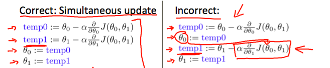
At each iteration j, one should simultaneously update the parameters θ_1, θ_2, …, θ_n. Updating a specific parameter prior to calculating another one on the j^{(th)} iteration would yield to a wrong implementation.
所以我们有假设函数,我们有一种方法可以衡量它与数据的匹配程度。现在我们需要估计假设函数中的参数。这就是梯度下降的地方。
想象一下,我们基于其字段 θ_0 和 θ_1 绘制我们的假设函数(实际上我们将成本函数绘制为参数估计的函数)。我们不是绘制 x 和 y 本身,而是绘制我们的假设函数的参数范围以及选择一组特定参数所产生的成本。
我们在 x 轴上设置 θ_0,在 y 轴上设置 θ_1,在垂直 z 轴上设置成本函数。我们的图上的点将是成本函数的结果,使用我们的假设和那些特定的 θ 参数。下图描绘了这样的设置。
当我们的成本函数位于图中凹坑的最底部时,即当它的值最小时,我们就知道我们已经成功了。红色箭头显示图表中的最小点。
我们这样做的方法是采用我们的成本函数的导数(一个函数的切线)。切线的斜率是该点的导数,它将为我们提供朝向的方向。我们在最陡下降的方向上降低成本函数。每个步骤的大小由参数 \alpha 确定,该参数称为学习速率。
例如,上图中每个 star 之间的距离表示由参数 \alpha 确定的步长。较小的 \alpha 将导致较小的步长,较大的 \alpha 会产生较大的步长。采取步骤的方向由 J(θ_0, θ_1) 的偏导数确定。根据图表的开始位置,可能会在不同的点上结束。上图显示了两个不同的起点,最终出现在两个不同的地方。
梯度下降算法是:
重复直到收敛:
在该情况下 j = 0,1 表示特征索引号。
在每次迭代 j 时,应该同时更新参数 θ_1, θ_2, …, θ_n。在 j^{(th)} 迭代中计算另一个参数之前更新特定参数将导致错误的实现。
九、梯度下降 - 说明
原文
In this video we explored the scenario where we used one parameter $θ_1$ and plotted its cost function to implement a gradient descent. Our formula for a single parameter was :Repeat until convergence:
Regardless of the slope’s sign for \frac{d}{dθ_1} J(θ_1), θ_1 eventually converges to its minimum value. The following graph shows that when the slope is negative, the value of θ_1 increases and when it is positive, the value of θ_1 decreases.
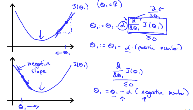
On a side note, we should adjust our parameter \alpha to ensure that the gradient descent algorithm converges in a reasonable time. Failure to converge or too much time to obtain the minimum value imply that our step size is wrong.
How does gradient descent converge with a fixed step size \alpha?
The intuition behind the convergence is that \frac{d}{dθ_1} J(θ_1) approaches 0 as we approach the bottom of our convex function. At the minimum, the derivative will always be 0 and thus we get:
在本视频中,我们探讨了使用一个参数θ_1并绘制其成本函数以实现梯度下降的场景。我们的单个参数公式是:
重复直到收敛:
无论 \frac{d}{dθ_1} J(θ_1) 的斜率符号如何,θ_1最终会收敛到其最小值。下图显示当斜率为负时,θ_1 的值增加,当它为正时,θ_1 的值减小。
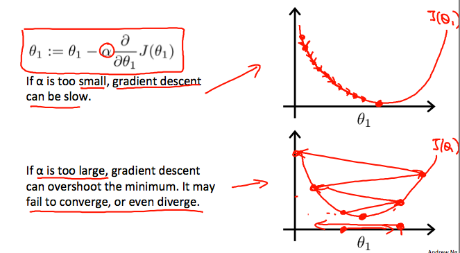
另外,我们应调整参数 \alpha 以确保梯度下降算法在合理的时间内收敛。没有收敛或太多时间来获得最小值意味着我们的步长是错误的。
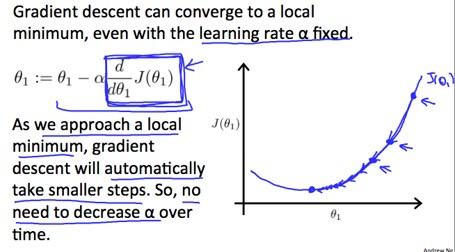
梯度下降如何与固定步长 \alpha 收敛?
收敛背后的直觉是当我们接近凸函数的底部时,\frac{d}{dθ_1} J(θ_1) 逼近 0。至少,导数总是 0,因此我们得到:
十、在线性回归中使用梯度下降
原文
When specifically applied to the case of linear regression, a new form of the gradient descent equation can be derived. We can substitute our actual cost function and our actual hypothesis function and modify the equation to:
where m is the size of the training set, θ_0 a constant that will be changing simultaneously with θ_1 and x_i, y_i are values of the given training set (data).
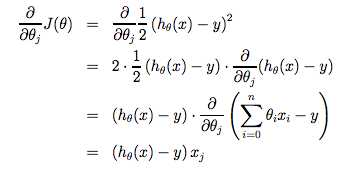
Note that we have separated out the two cases for θ_j into separate equations for θ_0 and θ_1; and that for θ_1 we are multiplying x_i at the end due to the derivative. The following is a derivation of \frac {\partial}{\partial \theta_j}J(\theta) for a single example:
The point of all this is that if we start with a guess for our hypothesis and then repeatedly apply these gradient descent equations, our hypothesis will become more and more accurate.
So, this is simply gradient descent on the original cost function J. This method looks at every example in the entire training set on every step, and is called batch gradient descent. Note that, while gradient descent can be susceptible to local minima in general, the optimization problem we have posed here for linear regression has only one global, and no other local, optima; thus gradient descent always converges (assuming the learning rate α is not too large) to the global minimum. Indeed, J is a convex quadratic function. Here is an example of gradient descent as it is run to minimize a quadratic function.
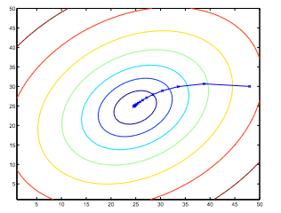
The ellipses shown above are the contours of a quadratic function. Also shown is the trajectory taken by gradient descent, which was initialized at (48,30). The x’s in the figure (joined by straight lines) mark the successive values of θ that gradient descent went through as it converged to its minimum.
当特别应用于线性回归的情况时,可以导出梯度下降方程的新形式。 我们可以用我们的实际成本函数和我们的实际假设函数代替并修改方程式
其中 m 是训练集的大小,θ_0 一个与 θ_1 同时变化的常数, 和 x_i, y_i 是给定训练集(数据)的值。
请注意,我们已将 θ_j 的两个案例分离为 θ_0, θ_1 的单独等式; 并且对于 θ_1 我们由于微分乘以 x_i 结尾。以下是 \frac {\partial}{\partial \theta_j}J(\theta) 的推导,用于单个示例:
所有这一切的要点是,如果我们开始猜测我们的假设,然后重复应用这些梯度下降方程,我们的假设将变得越来越准确。
因此,这只是原始成本函数 J 的梯度下降。该方法在每个步骤中查看整个训练集中的每个示例,并称为 批量梯度下降。 请注意,虽然梯度下降一般可以容易受到局部最小值的影响,但我们在这里为线性回归提出的优化问题只有一个全局,而没有其他局部最优; 因此,梯度下降总是收敛(假设学习率 α 不是太大)到全局最小值。 实际上,J 是凸二次函数。 下面是梯度下降的示例,因为它是为了最小化二次函数而运行的。
上面显示的椭圆是二次函数的轮廓。 还示出了梯度下降所采用的轨迹,其在 (48,30) 处初始化。 图中的 x(由直线连接)标记了渐变下降经历的 θ 的连续值,当它收敛到其最小值时。
十一、练习 2
原文
Consider the problem of predicting how well a student does in her second year of college/university, given how well she did in her first year.
Specifically, let x be equal to the number of
Agrades (including A-. A and A+ grades) that a student receives in their first year of college (freshmen year). We would like to predict the value of y, which we define as the number ofAgrades they get in their second year (sophomore year).Here each row is one training example. Recall that in linear regression, our hypothesis is h_\theta(x) = \theta_0 + \theta_1x, and we use m to denote the number of training examples.
x y 3 2 1 2 0 1 4 3 For the training set given above (note that this training set may also be referenced in other questions in this quiz), what is the value of m? In the box below, please enter your answer (which should be a number between
0and10).
Consider the following training set of m = 4 training examples:
x y 1 0.5 2 1 4 2 0 0 Consider the linear regression model h_θ(x) = θ_0 + θ_1x. What are the values of θ_0 and θ_1 that you would expect to obtain upon running gradient descent on this model? (Linear regression will be able to fit this data perfectly.)
- a. θ_0 = 0, θ_1 = 0.5
- b. θ_0 = 1, θ_1 = 0.5
- c. θ_0 = 1, θ_1 = 1
- d. θ_0 = 0.5, θ_1 = 0.5
- e. θ_0 = 0.5, θ_1 = 0
- Suppose we set θ_0 = -1, θ_1 = 0.5. What is h_θ(4)?
Let f be some function so that f(θ_0, θ_1) outputs a number.
For this problem, f is some arbitrary/unknown smooth function (not necessarily the cost function of linear regression, so f may have local optima).
Suppose we use gradient descent to try to minimize f(θ_0, θ_1) as a function of θ_0 and θ_1.
Which of the following statements are true? (Check all that apply.)
- a. If the learning rate is too small, then gradient descent may take a very long time to converge.
- b. Even if the learning rate \alpha is very large, every iteration of gradient descent will decrease the value of f(\theta_0, \theta_1).
- c. If \theta_0 and \theta_1 are initialized so that \theta_0 = \theta_1, then by symmetry (because we do simultaneous updates to the two parameters), after one iteration of gradient descent, we will still have \theta_0 = \theta_1.
- d. If \theta_0 and \theta_1 are initialized at a local minimum, then one iteration will not change their values.
Suppose that for some linear regression problem (say, predicting housing prices as in the lecture), we have some training set, and for our training set we managed to find some θ_0, θ_1 such that J(θ_0, θ_1) = 0.
Which of the statements below must then be true? (Check all that apply.)
- a. Gradient descent is likely to get stuck at a local minimum and fail to find the global minimum.
- b. For this to be true, we must have \theta_0 = 0 and \theta_1 = 0 so that h_\theta(x) = 0
- c. Our training set can be fit perfectly by a straight line, i.e., all of our training examples lie perfectly on some straight line.
- d. For this to be true, we must have y^{(i)} = 0 for every value of i = 1, 2, …, m$.
考虑一下学生在大学二年级学习成绩的问题,考虑到她在第一年的表现如何。
具体来说,让 x 等于学生在大学第一年(新生年)收到的
A等级(包括A-,A和A+等级)的数量。 我们想预测y的值,我们将其定义为他们在第二年(大二)获得的A等级的数量。这里每行都是一个训练示例。 回想一下,在线性回归中,我们的假设是 h_\theta(x) = \theta_0 + \theta_1x,我们使用 m 来表示训练样例的数量。
x y 3 2 1 2 0 1 4 3 对于上面给出的训练集(请注意,此训练集也可以在本测验中的其他问题中引用),m 的值是多少? 在下面的框中,请输入您的答案(应该是
0和10之间的数字)。
考虑以下 m = 4 训练示例的训练集:
x y 1 0.5 2 1 4 2 0 0 考虑线性回归模型 h_θ(x) = θ_0 + θ_1 x。在此模型上运行梯度下降时,您期望得到的 θ_0 和 θ_1 的值是多少? (线性回归将能够完美地拟合这些数据。)
- a. θ_0 = 0, θ_1 = 0.5
- b. θ_0 = 1, θ_1 = 0.5
- c. θ_0 = 1, θ_1 = 1
- d. θ_0 = 0.5, θ_1 = 0.5
- e. θ_0 = 0.5, θ_1 = 0
- 假设我们设置 θ_0 = -1, θ_1 = 0.5。 什么是 h_θ(4)?
让 f 成为某个函数,以便 f(θ_0, θ_1) 输出一个数字。
对于这个问题,f 是一些任意/未知的平滑函数(不一定是线性回归的代价函数,因此 f 可能具有局部最优)。
假设我们使用梯度下降来尝试最小化 f(θ_0, θ_1) 作为 θ_0 和 θ_1 的函数。
以下哪项陈述属实? (选择所有正确的选项。)
- a. 如果学习速率太小,则梯度下降可能需要很长时间才能收敛。
- b .即使学习率 \alpha 非常大,每次梯度下降迭代都会减少 f(\theta_0, \theta_1) 的值。
- c. 如果 \theta_0 和 \theta_1 被初始化以便 \theta_0 = \theta_1,那么通过对称(因为我们同时更新这两个参数),经过一次梯度下降迭代后,我们仍然会有 \theta_0 = \theta_1。
- d. 如果 \theta_0 和 \theta_1 初始化为局部最小值,则下一次迭代不会更改其值。
假设对于一些线性回归问题(比如在讲座中预测住房价格),我们有一些训练集,对于我们的训练集,我们设法找到一些 θ_0, θ_1,使得 J(θ_0, θ_1) = 0。
那么下面哪个陈述必须是真的?(选择所有正确的选项)
- a. 梯度下降可能会陷入局部最小值并且无法找到全局最小值。
- b. 为此,我们必须要 \theta_0 = 0 和 \theta_1 = 0 以便 h_\theta(x) = 0
- c. 我们的训练组可以通过直线完美贴合,即我们所有的训练样例都完美地位于某条直线上。
- d. 为此,对于 i = 1, 2, …, m 的每个值,我们必须有 y^{(i)} = 0。
答案
4m = 4 即为样本数量。
a代入公式 h_θ(x) = θ_0 + θ_1x 即可。
1把 θ_0 = -1, θ_1 = 0.5, x = 4 代入公式 h_θ(4) = -1 + 0.5 * 4 = 1。
a, d
cJ(θ_0, θ_1) = 0 代表所有的样本都能与该线性函数上的点完美贴合。
十二、专有词
机器学习定义
| abbreviate | original | description |
|---|---|---|
| T | task | 任务 |
| E | experience | 经验 |
| P | probability | 概率 |
几种算法
| abbreviate | original | description |
|---|---|---|
| supervised learning | - | 监督学习 |
| unsupervised learning | - | 无监督学习 |
| classification | - | 分类 |
| regression | - | 回归 |
线性回归
| abbreviate | original | description |
|---|---|---|
| m | number of tranining examples | 训练级数量 |
| x | input variable / features | 输入变量 / 特征 |
| y | output variable / target variable | 输出变量 / 目标变量 |
| (x, y) | - | 一个训练集样本 |
| (x(i), y(i)) | - | 第 i 个训练集样本,(i) 为下标 |
十三、数学补课
10.1 ∑ 的意义
在很多算法的文章书籍中能够见到很多 \displaystyle \sum_{i=0}^{100}(h(i)) 这样的数学表达式,但是我因为数学没好好学各种符号根本不认识。
∑ 代表求和的意思,和 math.Sum 类似但是不仅限于求和,它的下标代表了变量的起始,上标代表的声明的结束。
例如 \displaystyle \sum_{i=0}^{100}(h(i)) 可以转换为代码:
| |
自然上面的 \displaystyle \sum _{i=1}^m 代表的是样本下标从 1 开始到 m 结束,也就是遍历所有样本,注意数学公式的下标 i 与编程的起始定义不同,数学的下标 i 起始为 1。