机器学习第三周
文章目录
【注意】最后更新于 October 5, 2023,文中内容可能已过时,请谨慎使用。
前言
继续上一篇的的学习, 这一篇继续第三周的学习进度,使用逻辑回归来做分类。
一、分类
原文
To attempt classification, one method is to use linear regression and map all predictions greater than 0.5 as a 1 and all less than 0.5 as a 0. However, this method doesn’t work well because classification is not actually a linear function.
The classification problem is just like the regression problem, except that the values we now want to predict take on only a small number of discrete values. For now, we will focus on the binary classification problem in which y can take on only two values, 0 and 1. (Most of what we say here will also generalize to the multiple-class case.) For instance, if we are trying to build a spam classifier for email, then x^(i) may be some features of a piece of email, and y may be 1 if it is a piece of spam mail, and 0 otherwise. Hence, y∈{0,1}. 0 is also called the negative class, and 1 the positive class, and they are sometimes also denoted by the symbols - and +. Given x^(i), the corresponding y^(i) is also called the label for the training example.
要尝试分类,一种方法是使用线性回归并将所有大于 0.5 的预测映射为 1 并将所有小于 0.5 的预测映射为 0。但是,此方法效果不佳,因为分类实际上不是线性函数。
分类问题就像回归问题一样,除了我们现在要预测的值仅包含少量离散值。现在,我们将重点讨论二进制分类问题,其中 y 只能采用两个值 0 和 1。(我们在这里所说的大多数内容也将推广到多类情况。)例如,如果我们尝试要为电子邮件构建垃圾邮件分类器,则 x^(i) 可能是一封电子邮件的某些功能,如果它是一封垃圾邮件,则 y 为 1,否则为 0。因此,y∈{0,1}。 0 也称为否定类,1 也称为正类,有时也用符号 - 和 + 表示。给定 x^(i),相应的 y^(i) 为也称为培训示例的标签。
二、假设表示
原文
We could approach the classification problem ignoring the fact that y is discrete-valued, and use our old linear regression algorithm to try to predict y given x. However, it is easy to construct examples where this method performs very poorly. Intuitively, it also doesn’t make sense for h_θ(x) to take values larger than 1 or smaller than 0 when we know that y∈{0, 1}. To fix this, let’s change the form for our hypotheses h_θ(x) to satisfy 0 ≤ h_θ(x) ≤ 10. This is accomplished by plugging θ^Tx into the Logistic Function.
Our new form uses the “Sigmoid Function,” also called the “Logistic Function”:
The following image shows us what the sigmoid function looks like:
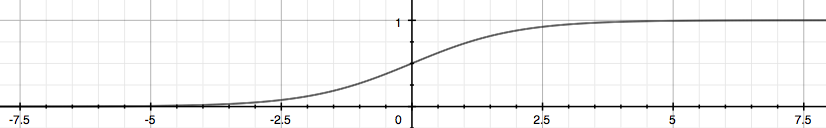
The function g(z), shown here, maps any real number to the (0, 1) interval, making it useful for transforming an arbitrary-valued function into a function better suited for classification.
h_θ(x) will give us the probability that our output is 1. For example, h_θ(x)=0.7 gives us a probability of 70% that our output is 1. Our probability that our prediction is 0 is just the complement of our probability that it is 1 (e.g. if probability that it is 1 is 70%, then the probability that it is 0 is 30%).
我们可以忽略 y 是离散值这一事实来处理分类问题,并使用我们的旧线性回归算法尝试在给定 x 的情况下预测 y。 但是,很容易构造这种方法效果很差的示例。 直观地讲,当我们知道 y∈{0,1} 时,h_θ(x)取大于 1 或小于 0 的值也没有意义。 为了解决这个问题,让我们更改假设 h_θ(x) 的形式,使其满足 0 ≤ h_θ(x) ≤ 10。 这是通过将 θ^Tx 插入逻辑函数来完成的。
我们的新形式使用 Sigmoid函数,也称为 Logistic函数:
下图显示了 Logistic函数 的外观:
此处显示的函数 g(z) 将任何实数映射到 (0, 1) 区间,这对于将任意值函数转换为更适合分类的函数很有用。
h_θ(x) 将给我们输出为 1 的概率。例如,h_θ(x) = 0.7给我们将输出为 1 的概率为 70%。我们预测为 0 的概率就是它是 1 的概率的补码(例如,如果它是 1 的概率是 70%,那么它是 0 的概率是 30%)。
三、决策边界
原文
In order to get our discrete 0 or 1 classification, we can translate the output of the hypothesis function as follows:
The way our logistic function g behaves is that when its input is greater than or equal to zero, its output is greater than or equal to 0.5:
Remember.
So if our input to g is θ^TX, then that means:
From these statements we can now say:
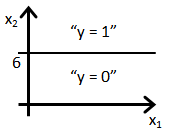
The decision boundary is the line that separates the area where y = 0 and where y = 1. It is created by our hypothesis function.
Example:
In this case, our decision boundary is a straight vertical line placed on the graph where x1 = 5, and everything to the left of that denotes y = 1, while everything to the right denotes y = 0.
Again, the input to the sigmoid function g(z) (e.g. θ^TX doesn’t need to be linear, and could be a function that describes a circle (e.g. z = θ_0 + θ_1x_1^2 + θ_2x_2^2) or any shape to fit our data.
为了获得离散的 0 或 1 分类,我们可以将假设函数的输出转换如下:
我们的逻辑函数 g 的行为方式是,当其输入大于或等于零时,其输出大于或等于 0.5:
记住。
因此,如果我们对 g 的输入是 θ^TX,则意味着:
从这些语句中,我们现在可以说:
决策边界 是分隔 y = 0 和 y = 1 区域的线。它是由我们的假设函数创建的。
Example:
在这种情况下,我们的决策边界是放置在图形上的垂直直线,其中 x1 = 5,其中左边的所有内容表示 y = 1,而右边的所有内容表示 y = 0。
同样,Logistic函数 g(z) 的输入(例如 θ^TX 不需要是线性的,可以是描述圆的函数(例如 z=θ_0 + θ_1x_1^2 + θ_2x_2^2)或任何适合我们数据的形状。
四、分类的代价函数
原文
We cannot use the same cost function that we use for linear regression because the Logistic Function will cause the output to be wavy, causing many local optima. In other words, it will not be a convex function.
Instead, our cost function for logistic regression looks like:
Similarly, when y = 0, we get the following plot for J(θ) vs h_θ(x):
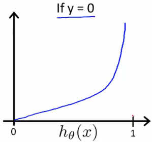
If our correct answer ‘y’ is 0, then the cost function will be 0 if our hypothesis function also outputs 0. If our hypothesis approaches 1, then the cost function will approach infinity.
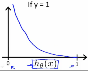
If our correct answer ‘y’ is 1, then the cost function will be 0 if our hypothesis function outputs 1. If our hypothesis approaches 0, then the cost function will approach infinity.
Note that writing the cost function in this way guarantees that J(θ) is convex for logistic regression.
我们不能使用与线性回归相同的成本函数,因为逻辑函数将导致输出波动,从而导致许多局部最优。 换句话说,它将不是凸函数。
相反,我们用于逻辑回归的成本函数如下所示:
同样,当 y = 0 时,我们得到 J(θ) vs h_θ(x) 的以下图:
如果我们正确的答案 y 为 0,那么如果我们的假设函数也输出 0,则成本函数将为 0。如果我们的假设接近 1,则成本函数将接近无穷大。
如果我们正确的答案 y 为 1,那么如果我们的假设函数输出为 1,则成本函数将为 0。如果我们的假设接近 0,则成本函数将接近无穷大。
请注意,以这种方式编写成本函数可确保 J(θ) 对于逻辑回归是凸的。
五、简化的成本函数和梯度下降
原文
We can compress our cost function’s two conditional cases into one case:
Notice that when y is equal to 1, then the second term (1-y)\log(1-h_\theta(x)) will be zero and will not affect the result. If y is equal to 0, then the first term -y \log(h_\theta(x)) will be zero and will not affect the result.
We can fully write out our entire cost function as follows:
A vectorized implementation is:
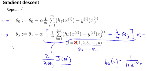
Gradient Descent
Remember that the general form of gradient descent is:
We can work out the derivative part using calculus to get:
Notice that this algorithm is identical to the one we used in linear regression. We still have to simultaneously update all values in \theta.
A vectorized implementation is:
我们可以将成本函数的两个条件情况压缩为一个情况:
请注意,当 y 等于 1 时,第二项 (1-y)\log(1-h_\theta(x)) 将为零,并且不会影响结果。 如果 y 等于 0,则第一项 -y \log(h_\theta(x)) 将为零,并且不会影响结果。
我们可以完全写出整个成本函数,如下所示:
向量化的实现是:
梯度下降
请记住,梯度下降的一般形式是:
我们可以使用微积分计算出导数部分,从而得到:
注意,该算法与我们在线性回归中使用的算法相同。 我们仍然必须同时更新 \theta 中的所有值。
向量化的实现是:
六、高级优化
原文
Conjugate gradient, BFGS, and L-BFGS are more sophisticated, faster ways to optimize θ that can be used instead of gradient descent. We suggest that you should not write these more sophisticated algorithms yourself (unless you are an expert in numerical computing) but use the libraries instead, as they’re already tested and highly optimized. Octave provides them.
We first need to provide a function that evaluates the following two functions for a given input value θ:
We can write a single function that returns both of these:
| |
Then we can use octave’s fminunc() optimization algorithm along with the optimset() function that creates an object containing the options we want to send to fminunc(). (Note: the value for MaxIter should be an integer, not a character string - errata in the video at 7:30)
| |
We give to the function fminunc() our cost function, our initial vector of theta values, and the options object that we created beforehand.
共轭梯度(Conjugate gradient),BFGS 和 L-BFGS 是优化 θ 的更复杂,更快速的方法,可用于替代梯度下降。 我们建议您不要自己编写这些更复杂的算法(除非您是数值计算方面的专家),而应改用这些库,因为它们已经过测试和高度优化。 Octave 提供它们。
我们首先需要提供一个函数,该函数针对给定的输入值 θ 评估以下两个函数:
我们可以编写一个返回这两个函数的函数:
| |
然后,我们可以使用 octave 的 fminunc() 优化算法以及 optimset() 函数,该函数创建一个对象,其中包含要发送给 fminunc() 的选项。(注意:MaxIter 的值应该是整数,而不是字符串-视频在 7:30 时显示是错误的)
| |
我们给函数 fminunc() 提供我们的成本函数,\theta 值的初始向量以及我们预先创建的 options 对象。
七、多类别分类
原文
Now we will approach the classification of data when we have more than two categories. Instead of y = {0,1} we will expand our definition so that y = {0,1…n}.
Since y = {0,1…n}, we divide our problem into n+1 (+1 because the index starts at 0) binary classification problems; in each one, we predict the probability that ‘y’ is a member of one of our classes.
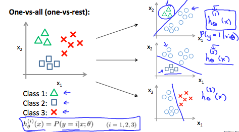
We are basically choosing one class and then lumping all the others into a single second class. We do this repeatedly, applying binary logistic regression to each case, and then use the hypothesis that returned the highest value as our prediction.
The following image shows how one could classify 3 classes:
To summarize:
Train a logistic regression classifier h_θ(x) for each class to predict the probability that y = i.
To make a prediction on a new x, pick the class that maximizes h_θ(x)
现在,当我们具有两个以上类别时,将对数据进行分类。 代替 y = {0,1},我们将扩展定义,以便 y = {0,1…n}。
由于 y = {0,1…n},我们将问题分为 n + 1(+1,因为索引从 0 开始)二进制分类问题。 在每一个类别中,我们都预测 y 是我们其中一个类别的成员的概率。
我们基本上是选择一个分类,然后将所有其他分类合并为一个第二分类。 我们反复进行此操作,对每种情况应用二元 logistic 回归,然后使用返回最高值的假设作为我们的预测。
下图显示了如何对 3 个类别进行分类:
总结一下:
为每个类训练一个逻辑回归分类器 h_θ(x) 来预测 y = i 的概率。
要对新 x 进行预测,请选择最大化 h_θ(x) 的类型。
八、测验
原文
- Suppose that you have trained a logistic regression classifier, and it outputs on a new example x a prediction h_θ(x) = 0.2. This means (check all that apply):
- a. Our estimate for P(y=1|x;\theta) is 0.2.
- b. Our estimate for P(y=0|x;\theta) is 0.2.
- a. Our estimate for P(y=1|x;\theta) is 0.8.
- a. Our estimate for P(y=0|x;\theta) is 0.8.
- Suppose you have the following training set, and fit a logistic regression classifier h_\theta(x) = g(\theta_0 + \theta_1x_1 + \theta_2 x_2).
| x1 | x2 | y |
|---|---|---|
| 1 | 0.5 | 0 |
| 1 | 1.5 | 0 |
| 2 | 1 | 1 |
| 3 | 1 | 0 |
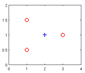
Which of the following are true? Check all that apply.
- a. J(\theta) will be a convex function, so gradient descent should converge to the global minimum.
- b. Adding polynomial features (e.g., instead using h_\theta(x) = g(\theta_0 + \theta_1x_1 + \theta_2 x_2 + \theta_3 x_1^2 + \theta_4 x_1 x_2 + \theta_5 x_2^2) ) could increase how well we can fit the training data.
- c. The positive and negative examples cannot be separated using a straight line. So, gradient descent will fail to converge.
- d. Because the positive and negative examples cannot be separated using a straight line, linear regression will perform as well as logistic regression on this data.
- For logistic regression, the gradient is given by \frac{\partial}{\partial \theta_j} J(\theta) =\frac{1}{m}\sum_{i=1}^m{ (h_\theta(x^{(i)}) - y^{(i)}) x_j^{(i)}}. Which of these is a correct gradient descent update for logistic regression with a learning rate of α? Check all that apply.
- a. \theta := \theta - \alpha \frac{1}{m} \sum_{i=1}^m{ \left(\theta^T x - y^{(i)}\right) x^{(i)}}.
- b. \theta_j := \theta_j - \alpha \frac{1}{m} \sum_{i=1}^m{ (h_\theta(x^{(i)}) - y^{(i)}) x_j^{(i)}} (simultaneously update for all j).
- c. \theta_j := \theta_j - \alpha \frac{1}{m} \sum_{i=1}^m{ (h_\theta(x^{(i)}) - y^{(i)}) x^{(i)}} (simultaneously update for all j).
- d. \theta_j := \theta_j - \alpha \frac{1}{m} \sum_{i=1}^m{ \left(\frac{1}{1 + e^{-\theta^T x^{(i)}}} - y^{(i)}\right) x_j^{(i)}} (simultaneously update for all j).
- Which of the following statements are true? Check all that apply.
- a. Since we train one classifier when there are two classes, we train two classifiers when there are three classes (and we do one-vs-all classification).
- b. The one-vs-all technique allows you to use logistic regression for problems in which each y^{(i)} comes from a fixed, discrete set of values.
- c. The cost function J(\theta) for logistic regression trained with m \geq 1 examples is always greater than or equal to zero.
- d. For logistic regression, sometimes gradient descent will converge to a local minimum (and fail to find the global minimum). This is the reason we prefer more advanced optimization algorithms such as fminunc (conjugate gradient/BFGS/L-BFGS/etc).
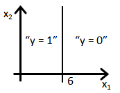
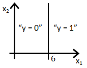
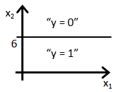
- Suppose you train a logistic classifier h_\theta(x) = g(\theta_0 + \theta_1x_1 + \theta_2 x_2). Suppose \theta_0 = - 6, \theta_1 = 1, \theta_2 = 0. Which of the following figures represents the decision boundary found by your classifier?
- a. Figure:
- b. Figure:
- c. Figure:
- d. Figure:
- 假设您已经训练了逻辑回归分类器,并且在新示例 x 上输出了预测 h_θ(x) = 0.2。 这意味着(多选)
- a. 我们对 P(y=1|x;\theta) 的估计为 0.2。
- b. 我们对 P(y=0|x;\theta) 的估计为 0.2。
- c. 我们对 P(y=1|x;\theta) 的估计为 0.8。
- d. 我们对 P(y=0|x;\theta) 的估计为 0.8。
- 假设您具有以下训练集,并拟合逻辑回归分类器 h_\theta(x) = g(\theta_0 + \theta_1x_1 + \theta_2 x_2)。
| x1 | x2 | y |
|---|---|---|
| 1 | 0.5 | 0 |
| 1 | 1.5 | 0 |
| 2 | 1 | 1 |
| 3 | 1 | 0 |
以下哪项是正确的?(多选)
- a. J(\theta) 将是一个凸函数,因此梯度下降应收敛到全局最小值。
- b. 添加多项式特征 (例如,改为使用 h_\theta(x) = g(\theta_0 + \theta_1x_1 + \theta_2 x_2 + \theta_3 x_1^2 + \theta_4 x_1 x_2 + \theta_5 x_2^2)) 可能会增加我们拟合训练数据的能力。
- c. 正例和负例不能使用直线分开。因此,梯度下降将无法收敛。
- d. 因为正和负的例子不能用直线分开,线性回归将执行以及该数据逻辑回归。
- 对于逻辑回归,梯度为 \frac{\partial}{\partial \theta_j} J(\theta) =\frac{1}{m}\sum_{i=1}^m{ (h_\theta(x^{(i)}) - y^{(i)}) x_j^{(i)}}。 以下哪项是学习速率为 α 的逻辑回归的正确梯度下降更新?(多选)
- a. \theta := \theta - \alpha \frac{1}{m} \sum_{i=1}^m{ \left(\theta^T x - y^{(i)}\right) x^{(i)}}.
- b. \theta_j := \theta_j - \alpha \frac{1}{m} \sum_{i=1}^m{ (h_\theta(x^{(i)}) - y^{(i)}) x_j^{(i)}} (同时更新所有 j).
- c. \theta_j := \theta_j - \alpha \frac{1}{m} \sum_{i=1}^m{ (h_\theta(x^{(i)}) - y^{(i)}) x^{(i)}} (同时更新所有 j).
- d. \theta_j := \theta_j - \alpha \frac{1}{m} \sum_{i=1}^m{ \left(\frac{1}{1 + e^{-\theta^T x^{(i)}}} - y^{(i)}\right) x_j^{(i)}} (同时更新所有 j).
- 下列哪个陈述是正确的?(多选)
- a. 由于我们在两个类别时训练一个分类器,因此在三个类别时我们训练两个分类器(并且我们进行一对多分类)。
- b. 一对多 技术使您可以将 逻辑回归(logistic regression) 用于问题中,其中每个 y^{(i)} 来自一组固定的离散值。
- c. 用 m \geq 1 示例训练的 逻辑回归(logistic regression) 的成本函数 J(\theta) 始终大于或等于零。
- d. 对于 逻辑回归(logistic regression),有时梯度下降将收敛到局部最小值(并且找不到全局最小值)。 这就是我们偏爱更高级的优化算法例如 fminunc(共轭梯度/BFGS/L-BFGS/etc) 的原因。
- 假设您训练了逻辑分类器 h_\theta(x) = g(\theta_0 + \theta_1x_1 + \theta_2 x_2)。 假设 \theta_0 = - 6, \theta_1 = 1, \theta_2 = 0。 以下哪个数字代表您的分类器找到的决策边界?
- a. Figure:
- b. Figure:
- c. Figure:
- d. Figure:
答案
a, da, b样本数量少所以肯定只有一个最优解,使用多项式特征能够更好的拟合数据集。a, b, db 是标准算式,a 是矩阵算式。b, c对于逻辑分类y的种类大于2需要的分类器数量为y。使用更高级的算法并不能避免出现局部最优解的问题。b如果是 \theta_0 = - 6, \theta_1 = 0, \theta_2 = 1 需要选d。
九、过度拟合的问题
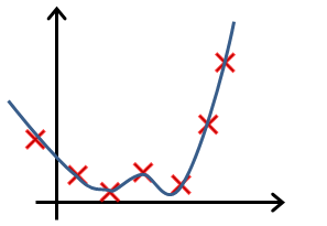
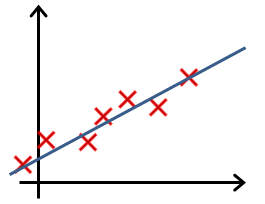
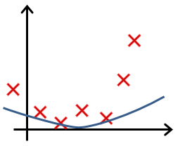
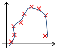
Consider the problem of predicting y from x ∈ R. The leftmost figure below shows the result of fitting a y = θ_0 + θ_1x to a dataset. We see that the data doesn’t really lie on straight line, and so the fit is not very good.
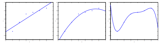
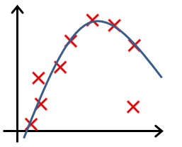
Instead, if we had added an extra feature x^2, and fit y = \theta_0 + \theta_1x + \theta_2x^2, then we obtain a slightly better fit to the data (See middle figure). Naively, it might seem that the more features we add, the better. However, there is also a danger in adding too many features: The rightmost figure is the result of fitting a 5^{th} order polynomial y = \sum_{j=0} ^5 \theta_j x^j. We see that even though the fitted curve passes through the data perfectly, we would not expect this to be a very good predictor of, say, housing prices (y) for different living areas (x). Without formally defining what these terms mean, we’ll say the figure on the left shows an instance of underfitting—in which the data clearly shows structure not captured by the model—and the figure on the right is an example of overfitting.
Underfitting, or high bias, is when the form of our hypothesis function h maps poorly to the trend of the data. It is usually caused by a function that is too simple or uses too few features. At the other extreme, overfitting, or high variance, is caused by a hypothesis function that fits the available data but does not generalize well to predict new data. It is usually caused by a complicated function that creates a lot of unnecessary curves and angles unrelated to the data.
This terminology is applied to both linear and logistic regression. There are two main options to address the issue of overfitting:
- Reduce the number of features:
- Manually select which features to keep.
- Use a model selection algorithm (studied later in the course).
- Regularization:
- Keep all the features, but reduce the magnitude of parameters θ_j.
- Regularization works well when we have a lot of slightly useful features.
十、在代价函数里使用正规化
Note: 5:18 - There is a typo. It should be \sum_{j=1}^{n} \theta _j ^2 instead of \sum_{i=1}^{n} \theta _j ^2
If we have overfitting from our hypothesis function, we can reduce the weight that some of the terms in our function carry by increasing their cost.
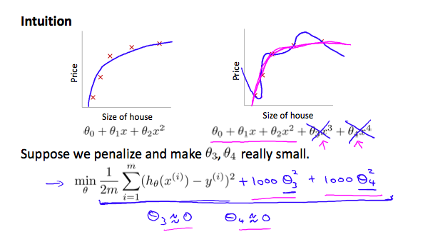
Say we wanted to make the following function more quadratic:
We’ll want to eliminate the influence of \theta_3x^3 and \theta_4x^4. Without actually getting rid of these features or changing the form of our hypothesis, we can instead modify our cost function:
We’ve added two extra terms at the end to inflate the cost of \theta_3 and \theta_4. Now, in order for the cost function to get close to zero, we will have to reduce the values of \theta_3 and \theta_4 to near zero. This will in turn greatly reduce the values of \theta_3x^3 and \theta_4x^4 in our hypothesis function. As a result, we see that the new hypothesis (depicted by the pink curve) looks like a quadratic function but fits the data better due to the extra small terms \theta_3x^3 and \theta_4x^4.
We could also regularize all of our theta parameters in a single summation as:
The \lambda, or lambda, is the regularization parameter. It determines how much the costs of our theta parameters are inflated.
Using the above cost function with the extra summation, we can smooth the output of our hypothesis function to reduce overfitting. If lambda is chosen to be too large, it may smooth out the function too much and cause underfitting. Hence, what would happen if \lambda = 0 or is too small ?
十一、正规化线性回归
Note: 8:43 - It is said that X is non-invertible if m \leq n. The correct statement should be that X is non-invertible if m < n, and may be non-invertible if m = n.
We can apply regularization to both linear regression and logistic regression. We will approach linear regression first. Gradient Descent
We will modify our gradient descent function to separate out \theta_0 from the rest of the parameters because we do not want to penalize \theta_0.
The term \frac{\lambda}{m}\theta_j performs our regularization. With some manipulation our update rule can also be represented as:
The first term in the above equation, 1 - \alpha\frac{\lambda}{m} will always be less than 1. Intuitively you can see it as reducing the value of \theta_j by some amount on every update. Notice that the second term is now exactly the same as it was before.
Normal Equation
Now let’s approach regularization using the alternate method of the non-iterative normal equation.
To add in regularization, the equation is the same as our original, except that we add another term inside the parentheses:
L is a matrix with 0 at the top left and 1’s down the diagonal, with 0’s everywhere else. It should have dimension (n+1)×(n+1). Intuitively, this is the identity matrix (though we are not including x_0), multiplied with a single real number \lambda.
Recall that if m < n, then X^TX is non-invertible. However, when we add the term λ⋅L, then X^TX + λ⋅L becomes invertible.
十二、正规化逻辑回归
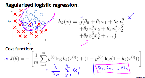
We can regularize logistic regression in a similar way that we regularize linear regression. As a result, we can avoid overfitting. The following image shows how the regularized function, displayed by the pink line, is less likely to overfit than the non-regularized function represented by the blue line:
Cost Function
Recall that our cost function for logistic regression was:
We can regularize this equation by adding a term to the end:
The second sum, \sum_{j=1}^n \theta_j^2 means to explicitly exclude the bias term, \theta_0. I.e. the θ vector is indexed from 0 to n (holding n+1 values, \theta_0 through \theta_n), and this sum explicitly skips \theta_0, by running from 1 to n, skipping 0. Thus, when computing the equation, we should continuously update the two following equations:
测验2
原文
---- You are training a classification model with logistic regression. Which of the following statements are true? Check all that apply.
- a. Adding a new feature to the model always results in equal or better performance on the training set.
- b. Introducing regularization to the model always results in equal or better performance on the training set.
- c. Introducing regularization to the model always results in equal or better performance on examples not in the training set.
- d. Adding many new features to the model helps prevent overfitting on the training set.
- Suppose you ran logistic regression twice, once with \lambda = 0, and once with \lambda = 1 .
One of the times, you got parameters \theta = \begin{bmatrix} 81.47 \newline 12.69 \end{bmatrix}, and the other time you got \theta = \begin{bmatrix} 13.01 \newline 0.91 \end{bmatrix}.
However, you forgot which value of \lambda corresponds to which value of \theta. Which one do you think corresponds to \lambda = 1?
- a. \theta = \begin{bmatrix} 81.47 \newline 12.69 \end{bmatrix}
- b. \theta = \begin{bmatrix} 13.01 \newline 0.91 \end{bmatrix}
- Which of the following statements about regularization are true? Check all that apply.
- a. Because logistic regression outputs values 0 \leq h_\theta(x) \leq 1, its range of output values can only be “shrunk” slightly by regularization anyway, so regularization is generally not helpful for it.
- b. Using too large a value of \lambda can cause your hypothesis to overfit the data; this can be avoided by reducing \lambda.
- c. Using a very large value of \lambda cannot hurt the performance of your hypothesis; the only reason we do not set \lambda to be too large is to avoid numerical problems.
- d. Consider a classification problem. Adding regularization may cause your classifier to incorrectly classify some training examples (which it had correctly classified when not using regularization, i.e. when \lambda = 0).
- In which one of the following figures do you think the hypothesis has overfit the training set?
- a. Figure:
- b. Figure:
- c. Figure:
- d. Figure:
- In which one of the following figures do you think the hypothesis has underfit the training set?
- a. Figure:
- b. Figure:
- c. Figure:
- d. Figure:
- 您正在使用逻辑回归训练分类模型。下列哪个陈述是正确的?选择所有对的选项。
- a. 向模型添加新特征总是可以使训练集具有相同或更好的性能。
- b. 向模型引入正规化总是会导致训练集具有相同或更好的性能。
- c. 向模型引入正规化总是会导致训练集中未包含的示例具有相同或更好的性能。
- d. 向模型添加许多新特征有助于防止训练集过拟合。
// a, c
- 假设您进行了两次逻辑回归,一次使用 \lambda = 0,一次使用 \lambda = 1。
一次,您有参数 \theta = \begin{bmatrix} 81.47 \newline 12.69 \end{bmatrix},而另一次,您有 \theta = \begin{bmatrix} 13.01 \newline 0.91 \end{bmatrix}。
但是,您忘记了 \lambda 的哪个值对应于 \theta 的哪个值。您认为哪一个对应于 \lambda = 1?
- a. \theta = \begin{bmatrix} 81.47 \newline 12.69 \end{bmatrix}
- b. \theta = \begin{bmatrix} 13.01 \newline 0.91 \end{bmatrix}
//b
- 下列有关正规化的哪些陈述是正确的? 选中所有适用。
- a. 由于逻辑回归输出值 0 \leq h_\theta(x) \leq1,无论如何,通过正则化只能稍微
缩小其输出值范围,因此正规化通常对此无济于事。 - b. 使用太大的 \lambda 值可能会导致您的假设过度拟合数据。这可以通过减少 \lambda 来避免。
- c. 使用非常大的 \lambda 值不会损害假设的执行;我们没有将 \lambda 设置得太大的唯一原因是为了避免数值问题。
- d. 考虑分类问题。 添加正则化可能会导致您的分类器对一些训练示例进行错误分类(当未使用正则化时,即 \lambda = 0 时,它已经正确分类了)。
// d
- 您认为以下哪个图中的假设与训练集过度拟合?
- a. Figure:
- b. Figure:
- c. Figure:
- d. Figure:
- 您认为以下哪个图中的假设不适合训练集?
- a. Figure:
- b. Figure:
- c. Figure:
- d. Figure: