机器学习第二周
文章目录
【注意】最后更新于 May 8, 2021,文中内容可能已过时,请谨慎使用。
前言
继续上一篇的的学习,这一篇继续第二周的学习进度, 主要内容为多特征,Octave 使用。
一、多个特征
原文
Note: [7:25 - θ^T is a 1 by (n+1) matrix and not an (n+1) by 1 matrix]
Linear regression with multiple variables is also known as multivariate linear regression.
We now introduce notation for equations where we can have any number of input variables.
The multivariable form of the hypothesis function accommodating these multiple features is as follows:
h_\theta (x) = \theta_0 + \theta_1 x_1 + \theta_2 x_2 + \theta_3 x_3 + \cdots + \theta_n x_n
In order to develop intuition about this function, we can think about θ_0 as the basic price of a house, θ_1 as the price per square meter, θ_2 as the price per floor, etc. x_1 will be the number of square meters in the house, x_2 the number of floors, etc.
Using the definition of matrix multiplication, our multivariable hypothesis function can be concisely represented as:
This is a vectorization of our hypothesis function for one training example; see the lessons on vectorization to learn more.
Remark: Note that for convenience reasons in this course we assume x_{0}^{(i)} = 1 \text{ for } (i\in { 1,\dots, m }). This allows us to do matrix operations with theta and x. Hence making the two vectors ‘\theta’ and x^{(i)} match each other element-wise (that is, have the same number of elements: n+1).]
Note: θ^T 是 1 * (n+1) 的矩阵(横)而不是 (n+1) * 1 的矩阵(纵)
具有多个变量的线性回归也称为 多元线性回归。
我们现在为方程式引入符号,其中我们可以有任意数量的输入变量。
适应这些多个特征的假设函数的多变量形式如下:
h_\theta (x) = \theta_0 + \theta_1 x_1 + \theta_2 x_2 + \theta_3 x_3 + \cdots + \theta_n x_n
为了发展关于这个功能的直觉,我们可以考虑 θ_0 作为房子的基本价格,θ_1 作为每平方米的价格,θ_2 作为每层的价格等等。x_1 将是房子里的平方米数,x_2 楼层数等。
使用矩阵乘法的定义,我们的多变量假设函数可以简洁地表示为:
这是一个训练例子的假设函数的矢量化;请参阅有关矢量化的课程以了解更多信息。
Remark: 请注意,为了方便起见,在本课程中我们假设 x_{0}^{(i)} = 1 \text{ for } (i\in { 1,\dots, m }). 这允许我们用 theta 和 x 进行矩阵运算。因此,使两个向量 ‘\theta’ 和 x^{(i)} 彼此元素匹配(即,具有相同数量的元素:n + 1)。
二、多个特征变量的梯度下降
原文
The gradient descent equation itself is generally the same form; we just have to repeat it for our n features:
In other words:
The following image compares gradient descent with one variable to gradient descent with multiple variables:
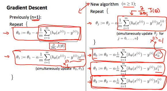
梯度下降方程本身通常是相同的形式。 我们只需要为我们的 n 个特征重复一下:
换句话说:
下图将具有一个特征变量的梯度下降与具有多个多个变量的梯度下降进行比较:
三、梯度下降实践 1 - 特征缩放
原文
Note: The average size of a house is 1000 but 100 is accidentally written instead
We can speed up gradient descent by having each of our input values in roughly the same range. This is because θ will descend quickly on small ranges and slowly on large ranges, and so will oscillate inefficiently down to the optimum when the variables are very uneven.
The way to prevent this is to modify the ranges of our input variables so that they are all roughly the same. Ideally:
These aren’t exact requirements; we are only trying to speed things up. The goal is to get all input variables into roughly one of these ranges, give or take a few.
Two techniques to help with this are feature scaling and mean normalization. Feature scaling involves dividing the input values by the range (i.e. the maximum value minus the minimum value) of the input variable, resulting in a new range of just 1. Mean normalization involves subtracting the average value for an input variable from the values for that input variable resulting in a new average value for the input variable of just zero. To implement both of these techniques, adjust your input values as shown in this formula:
Where μ_i is the average of all the values for feature (i) and s_i is the range of values (max - min), or s_i is the standard deviation.
Note that dividing by the range, or dividing by the standard deviation, give different results. The quizzes in this course use range - the programming exercises use standard deviation.
For example, if represents housing prices with a range of 100 to 2000 and a mean value of 1000, then, x_i := \dfrac{price-1000}{1900}.
Note: 房屋的平均大小为 1000,但也可故意写为 100
我们可以通过将每个输入值设置在大致相同的范围内来加快梯度下降的速度。 这是因为 θ 在小范围内会迅速下降,而在大范围内会缓慢下降,因此当变量非常不均匀时,会无效率地振荡到最佳状态。
防止这种情况的方法是修改输入变量的范围,以使它们都大致相同。理想的情况是:
这些不是确切的要求; 我们只是试图加快速度。 目标是使所有输入变量大致进入这些范围之一,给出或取几个。
两种有助于此目的的技术是 特征缩放 和 平均归一化。 特征缩放涉及将输入值除以输入变量的范围(即最大值减去最小值),从而得到新的范围仅为 1。平均归一化涉及从输入值的平均值中减去输入变量的平均值。 输入变量导致输入变量的新平均值仅为零。 要实现这两种技术,请按照以下公式调整输入值:
其中 μ_i 是特征 (i) 所有值的 平均值,而 s_i 是值的范围(最大值-最小值),或 s_i 是标准偏差。
请注意,除以范围或除以标准偏差会得出不同的结果。 本课程中的测验使用范围-编程练习使用标准偏差。
例如,如果代表的房价范围为 100 至 2000,平均值为 1000,则,x_i := \dfrac{price-1000}{1900}。
四、梯度下降实践 1 - 学习速率
原文
Note: the x-axis label in the right graph should be θ rather than No. of iterations
Debugging gradient descent. Make a plot with number of iterations on the x-axis. Now plot the cost function, J(θ) over the number of iterations of gradient descent. If J(θ) ever increases, then you probably need to decrease α.
Automatic convergence test. Declare convergence if J(θ) decreases by less than E in one iteration, where E is some small value such as 10^{-3}. However in practice it’s difficult to choose this threshold value.
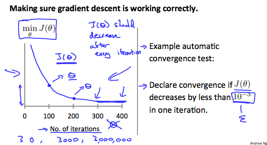
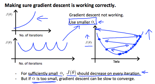
It has been proven that if learning rate α is sufficiently small, then J(θ) will decrease on every iteration.
To summarize:
If α is too small: slow convergence.
If α is too large: may not decrease on every iteration and thus may not converge.
Note: 右图中的 x 轴标签应为 θ 而不是迭代次数。
调试梯度下降。 绘制一个在 x 轴上具有迭代次数的图。 现在在梯度下降的迭代次数上绘制成本函数 J(θ)。 如果 J(θ) 曾经增加,那么您可能需要减少 α。
自动收敛测试。 如果 J(θ) 在一次迭代中减小的幅度小于 E,则声明收敛,其中 E 是一些小值,例如 10^{-3}。 但是实际上,很难选择此阈值。
已经证明,如果学习率 α 足够小,则 J(θ) 将在每次迭代中减小。
总结一下:
如果 α 太小:收敛缓慢。
如果 α 太大:可能不会在每次迭代中都减少,因此可能不会收敛。
五、特征和多项式的回归函数
原文
We can improve our features and the form of our hypothesis function in a couple different ways.We can combine multiple features into one. For example, we can combine x_1 and x_2 into a new feature x_3 by taking x_1⋅x_2.
Polynomial Regression
Our hypothesis function need not be linear (a straight line) if that does not fit the data well.
We can change the behavior or curve of our hypothesis function by making it a quadratic, cubic or square root function (or any other form).
For example, if our hypothesis function is h_\theta(x) = \theta_0 + \theta_1 x_1 then we can create additional features based on x_1, to get the quadratic function h_\theta(x) = \theta_0 + \theta_1 x_1 + \theta_2 x_1^2 or the cubic function h_\theta(x) = \theta_0 + \theta_1 x_1 + \theta_2 x_1^2 + \theta_3 x_1^3
In the cubic version, we have created new features x_2 and x_3 where x_2=x_1^2 and x_3=x_1^3.
To make it a square root function, we could do: h_\theta(x) = \theta_0 + \theta_1 x_1 + \theta_2 \sqrt{{x_1}}
One important thing to keep in mind is, if you choose your features this way then feature scaling becomes very important.
eg. if x_1 has range 1 - 1000 then range of x_1^2 becomes 1 - 1000000 and that of x_1^3 becomes 1 - 1000000000
我们可以通过几种不同的方式来改进我们的特征和假设函数的形式。
我们可以将多个功能组合为一个。例如,我们可以采用 x_1 ⋅ x_2,将 x_1 和 x_2 组合成一个新功能 x_3。
多项式回归
如果我们的假设函数不太适合数据的分布,则不必是线性的(直线)。
我们可以通过将其设为二次,三次或平方根函数(或任何其他形式)来更改假设函数的行为或曲线。
例如,如果我们的假设函数是 h_\theta(x) = \theta_0 + \theta_1 x_1,那么我们可以基于 x_1 创建其他特征,以获得二次函数 h_\theta(x) = \theta_0 + \theta_1 x_1 + \theta_2 x_1^2 或三次函数 h_\theta(x) = \theta_0 + \theta_1 x_1 + \theta_2 x_1^2 + \theta_3 x_1^3
在三次版本中,我们创建了新特征 x_2 和 x_3,其中 x_2 = x_1^2 和 x_3 = x_1^3。
要使它成为平方根函数,我们可以这样做:h_\theta(x) = \theta_0 + \theta_1 x_1 + \theta_2 \sqrt{x_1}
要记住的一件事是,如果以这种方式选择要素,则特征缩放变得非常重要。
例如。如果 x_1 的范围为 1-1000,则 x_1^2 的范围为 1-1000000,而 x_1^3 的范围为 1-1000000000
六、正规方程
原文
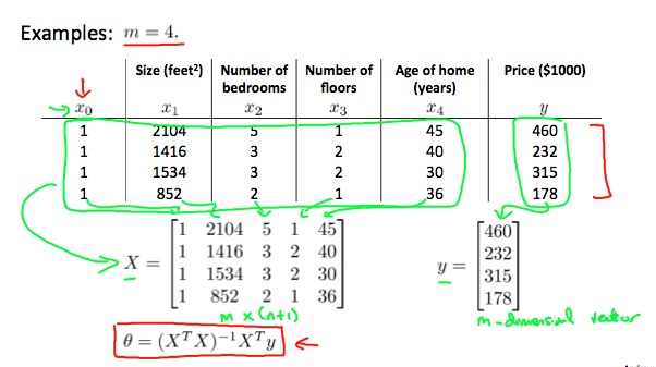
Note: he design matrix X (in the bottom right side of the slide) given in the example should have elements x with subscript 1 and superscripts varying from 1 to m because for all m training sets there are only 2 features x_0 and x_1; The X matrix is m by (n+1) and NOT n by n.
Gradient descent gives one way of minimizing J. Let’s discuss a second way of doing so, this time performing the minimization explicitly and without resorting to an iterative algorithm. In the “Normal Equation” method, we will minimize J by explicitly taking its derivatives with respect to the θj ’s, and setting them to zero. This allows us to find the optimum theta without iteration. The normal equation formula is given below:
| |
There is no need to do feature scaling with the normal equation.
The following is a comparison of gradient descent and the normal equation:
| Gradient Descent | Normal Equation |
|---|---|
| Need to choose alpha | No need to choose alpha |
| Needs many iterations | No need to iterate |
| O(kn^2) | O(n^3), need to calculate inverse of X^T X |
| Works well when n is large | Slow if n is very large |
With the normal equation, computing the inversion has complexity \mathcal{O}(n^3). So if we have a very large number of features, the normal equation will be slow. In practice, when n exceeds 10,000 it might be a good time to go from a normal solution to an iterative process.
Note: 在示例中给出的设计矩阵 X(在幻灯片的右下角)应具有元素 x,其下标 1 和上标的范围从 1 到 m,因为对于所有 m 个训练集,只有 2 个特征 x_0 和 x_1; X 矩阵的 m 乘 (n + 1),而不是 n * n。
梯度下降提供了一种最小化 J 的方法。让我们讨论这样做的第二种方法,这一次显式地执行最小化,而不求助于迭代算法。 在 正态方程 方法中,我们将通过显式地将其关于 θj 的导数并将其设置为零来最小化 J。 这使我们无需迭代即可找到最佳 θ。 正态方程公式如下:
octave 的代码公式
| |
正规方程无需使用特征缩放。
以下是梯度下降与正规方程的比较:
| 梯度下降 | 正规方程 |
|---|---|
| 需要选择 \alpha | 不需要选择 \alpha |
| 需要多次迭代 | 不需要进行迭代 |
| O(kn^2) | O(n^3), 需要计算逆 X^T X |
| 当 n 大时效果很好 | 如果 n 很大,则变慢 |
利用正规方程,计算反演的复杂度为 \mathcal{O}(n^3)。 因此,如果我们具有大量特征,则正常方程将变慢。 在实践中,当 n 超过 10,000 时,可能是从常规解转到迭代过程的好时机。
七、测验
原文
- Suppose m=4 students have taken some class, and the class had a midterm exam and a final exam. You have collected a dataset of their scores on the two exams, which is as follows:
| midterm exam | (midterm exam)^2 | final exam |
|---|---|---|
| 89 | 7921 | 96 |
| 72 | 5184 | 74 |
| 94 | 8836 | 87 |
| 69 | 4761 | 78 |
You’d like to use polynomial regression to predict a student’s final exam score from their midterm exam score. Concretely, suppose you want to fit a model of the form h_θ(x)=θ_0 + θ_1x1 + θ_2x2, where x_1 is the midterm score and x_2 is (midterm score)^2. Further, you plan to use both feature scaling (dividing by the “max-min”, or range, of a feature) and mean normalization. What is the normalized feature x_2^{(4)}? (Hint: midterm = 69, final = 78 is training example 4.) Please round off your answer to two decimal places and enter in the text box below.
- You run gradient descent for 15 iterations with α = 0.3 and compute J(θ) after each iteration. You find that the value of J(θ) decreases quickly then levels off. Based on this, which of the following conclusions seems most plausible?
- a. α = 0.3 is an effective choice of learning rate.
- b. Rather than use the current value of α, it’d be more promising to try a smaller value of α (say α = 0.1).
- c. Rather than use the current value of α, it’d be more promising to try a smaller value of α (say α = 1.0).
- Suppose you have m = 23 training examples with n = 5 features (excluding the additional all-ones feature for the intercept term, which you should add). The normal equation is \theta = (X^TX)^{-1}X^Ty. For the given values of m and n, what are the dimensions of θ, X, and y in this equation?
- a. X is 23\times6, y is 23\times1, θ is 6\times1
- b. X is 23\times5, y is 23\times1, θ is 5\times5
- c. X is 23\times6, y is 23\times6, θ is 6\times6
- d. X is 23\times5, y is 23\times1, θ is 5\times1
- Suppose you have a dataset with m=50 examples and n=15 features for each example. You want to use multivariate linear regression to fit the parameters θ to our data. Should you prefer gradient descent or the normal equation?
- a. Gradient descent, since it will always converge to the optimal α.
- b. Gradient descent, since (X^TX)^{-1} will be very slow to compute in the normal equation.
- c. The normal equation, since it provides an efficient way to directly find the solution.
- d. The normal equation, since gradient descent might be unable to find the optimal θ.
- Which of the following are reasons for using feature scaling?(many select)
- a. It prevents the matrix X^TX (used in the normal equation) from being non-invertable (singular/degenerate).
- b. It speeds up gradient descent by making it require fewer iterations to get to a good solution.
- c. It speeds up solving for \theta using the normal equation.
- d. It is necessary to prevent gradient descent from getting stuck in local optima.
- 假设 m = 4 个学生参加了某堂课,并且该班进行了期中考试和期末考试。 您已经收集了两次考试的分数数据集,如下所示:
| 期中考试 | \text{期中考试}^2 | 期末考试 |
|---|---|---|
| 89 | 7921 | 96 |
| 72 | 5184 | 74 |
| 94 | 8836 | 87 |
| 69 | 4761 | 78 |
您想使用多项式回归来根据学生的期中考试成绩来预测学生的期末考试成绩。 具体来说,假设您要拟合 h_θ(x)=θ_0+θ_1x1+θ_2x2 形式的模型,其中 x_1 是期中分数,x_2 是 \text{期中分数}^2。 此外,您计划同时使用特征缩放(除以特征的 max - min 或范围)和均值归一化。
什么是标准化特征 x_2^{(4)}? (提示:期中 = 69,期末 = 78是训练示例4。)请四舍五入到小数点后两位,然后在下面的文本框中输入。
- 您运行梯度下降 15 次迭代 α=0.3 并计算 每次迭代后的 J(θ)。 您发现 J(θ) 的值迅速下降,然后下降 关闭。 基于此,以下哪个结论似乎 最合理?
- a. α = 0.3 是学习率的有效选择。
- b. 与其使用 α 的当前值,不如尝试使用较小的 α 值(例如 α=0.1)。
- c. 与其使用 α 的当前值,不如尝试使用较大的 α 值(例如 α=1.0)。
- 假设您有 m=23 个训练示例,其中包含 n=5 个特征(不包括用于拦截项的附加全一功能,您应该添加该功能)。 正规方程为 \theta = (X ^ TX)^{-1}X ^ Ty。 对于给定的 m 和 n 值,方程中 θ,X 和 y 的尺寸分别是多少?
- a. X 是 23\times6, y 是 23\times1, θ 是 6\times1
- b. X 是 23\times5, y 是 23\times1, θ 是 5\times5
- c. X 是 23\times6, y 是 23\times6, θ 是 6\times6
- d. X 是 23\times5, y 是 23\times1, θ 是 5\times1
- 假设您有一个包含 m = 50 个示例和每个示例 n = 15 个特征的数据集。 您想使用多元线性回归将参数 θ 拟合到我们的数据中。 您应该选择
梯度下降还是正规方程?
- a. 梯度下降,因为它将始终收敛到最佳 α。
- b. 梯度下降,因为在正规方程中 (X ^ TX)^{-1} 的计算将非常缓慢。
- c. 正规方程,因为它提供了直接找到解的有效方法。
- d. 正规方程,因为梯度下降可能无法找到最佳的 θ。
- 以下哪些是使用特征缩放的原因?(多选)
- a. 这样可以防止矩阵 X^TX(在正常方程式中使用)不可逆(奇异/简并)。
- b. 它通过减少迭代次数来获得良好的解决方案,从而加快了梯度下降的速度。
- c. 它可以使用法线方程加快求解 \theta 的速度。
- d. 有必要防止梯度下降陷入局部最优状态。
答案
0.47(7921 + 5184 + 8836 + 4761) / 4 = 6675.5, 8836 - 4761 = 4075, \dfrac{4761 - 6675.5}{4075} = 0.4698159509202454.a, 刚好匹配就是快速计算出正确的值,太大 \theta 可能会出现增大,太小会出现 \theta 值的下降缓慢。acb, a: 特征缩放仅对梯度下降方程有效,c: 并不会加快线性方程,d: 特征缩放无法处理局部最优解。
八、Octave 使用
python 环境下需要导入以下库
| |
| 说明 | Octave | Python + Numpy + Matplotlib |
|---|---|---|
| 加 | 1 + 2 | 1 + 2 |
| 减 | 1 - 2 | 1 - 2 |
| 乘 | 1 * 2 | 1 * 2 |
| 除 | 1 / 2 | 1 / 2 |
| 幂 | 1 ^ 2 | 1 ** 2 |
| 抑制结果打印 | ${表达式}; | - |
| 逻辑或 | a || b | a or b |
| 逻辑与 | a && b | a and b |
| 位异或 | XOR(a, b) | a ^ b |
| 等于 | a == b | a == || is b |
| 不等于 | a ~= b | a != || not is b |
| 大于 | a > b | a > b |
| 小于 | a < b | a < b |
| 大于等于 | a >= b | a >= b |
| 小于等于 | a <= b | a <= b |
| 打印变量 | disp(a) | print(a) |
| 字符串格式化 | sprintf('%0.2f', a) | '%0.2f' % a |
| 创建矩阵 | a = [1 2; 3 4; 5 6] | a = np.array([(1, 2), (3, 4), (5, 6)] |
| 递进创建向量 | a = [1:0.1:2] | a = np.arange(1, 2 + 0.1, 0.1) |
| 填充创建矩阵 | a = 2 * ones(2, 3) | a = 2 * np.ones((2, 3), dtype=np.uint32) |
| 创建随机填充的矩阵 | a = rand(2, 3) | a = np.random.rand(2, 3) |
| 高斯分布矩阵 | a = randn(2, 3) | a = np.random.randn(2, 3) |
| 对角矩阵 | a = eye(3) | a = np.eye(3) |
| 矩阵大小 | sz = size(a) | sz = np.shape(a) |
| 加载磁盘上的数据 | load('file') | a = numpy.load('file') |
| 保存变量 | save 'file' a | numpy.save('file', a) |
| 保存变量到纯文本 | save 'file' a -ascii | numpy.savetxt('file', a) |
| 查看全部变量 | who | - |
| 查看全部变量详情 | whos | - |
| 清理变量 | clear a | - |
| 矩阵元素访问 | a(1, 1) | a[0][0] or a[0, 0] |
| 矩阵行访问 | a(1, :) | a[0] or a[0, :] |
| 矩阵列访问 | a(:, 1) | a[:, 0] |
| 矩阵限制列或行 | a(:, [1 2]) | a[:, (0, 1)] |
| 增加一列(合并列) | a = [a [8; 9]] | np.c_(a, np.array([[8, 9]]).T) |
| 增加一行(合并行) | a = [a; [8 9 10]] | np.r_(a, np.array([[8, 9, 10]])) |
| 矩阵转行向量 | a(:) | a.flatten() or a.ravel() |
| 矩阵乘法 | a .* b | a * b |
| 矩阵转置 | a' | a.T |
| 矩阵绝对值 | abs(a) | np.abs(a) |
| 矩阵平方根 | sqrt(a) | np.sqrt(a) |
| 矩阵对数 | log(a) | np.log(a) |
| 矩阵最大值 | max(a) | np.max(a) |
| 矩阵最小值 | min(a) | np.min(a) |
| 矩阵求和 | sum(a) | np.sum(a) |
| 矩阵求乘积 | prod(a) | np.prod(a) |
| 矩阵向下取整 | floor(a) | np.floor(a) |
| 矩阵向上取整 | ceil(a) | np.ceil(a) |
| 矩阵元素比较 | a > 1 | a > 1 |
| 矩阵根据比较结果矩阵过滤 | find(a >1) | a[a > 1] |
| 幻方矩阵 | magic(3) | 可自行实现 |
| 矩阵求逆 | pinv(a) | np.linalg.pinv(a) |
| 矩阵正弦函数 | sin(a) | np.sin(a) |
| 绘制线性函数 | polt(t, y1) | plt.polt(t, y1) |
| 绘制分布柱型图 | w = -6 + sqrt(10) * randn(1, 100);hist(w, 10) | w = -6 + math.sqrt(10) * np.random.randn(1, 100);plt.hist(w[0], 10) |
八、参考
- c-printf: c字符串格式化说明。
- numpy手册
- matplotlib手册
- scipy手册